Investigate and optimize the acoustic performance of porous and microperforate materials with acoustipy. Use the acoustic transfer matrix method to explore new material designs and identify unique properties of existing materials via inverse, indirect, and hybrid optimization schemes.
Installation
Create and activate a new virtual environment (recommended)
mkdir <your_env_name>
python -m venv .venv
cd .venv
(Windows) cd Scripts && activate.bat
(Linux) source bin/activate
Install from source
git clone https://github.com/jakep72/acoustipy.git
cd acoustipy
pip install -e .
pip install -r requirements.txt
Install from PyPI
pip install acoustipy
Basic Usage
Examples of most of the functionality of acoustipy can be found in the Examples section. The snippet below corresponds to the multilayer structure example and highlights a core feature of acoustipy -- the acoustic transfer matrix method.
from acoustipy import acousticTMM
# Create an AcousticTMM object, specifying a diffuse sound field at 20C
structure = AcousticTMM(incidence='Diffuse',air_temperature=20)
# Define the layers of the material using various models
layer1 = structure.Add_Resistive_Screen(thickness=1,flow_resistivity=100000,porosity=.86)
layer2 = structure.Add_DBM_Layer(thickness = 25.4,flow_resistivity=60000)
layer3 = structure.Add_Resistive_Screen(thickness = 1, flow_resistivity=500000,porosity=.75)
# Specify the material backing condition -- in this case a 400mm air gap
air = structure.Add_Air_Layer(thickness = 400)
# Build the total transfer matrix of the structure + air gap
transfer_matrix = structure.assemble_structure(layer1,layer2,layer3,air)
# Calculate the frequency dependent narrow band absorption coefficients
absorption = structure.absorption(transfer_matrix)
# Calculate the 3rd octave bands absorption coefficients
bands = structure.octave_bands(absorption)
# Calculate the four frequency average absorption
FFA = structure.FFA(bands)
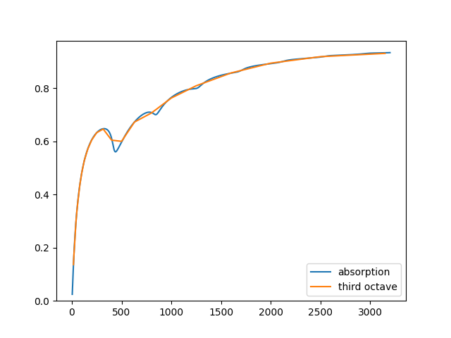
# Plot and display the narrow and 3rd band coefficients on the same figure
structure.plot_curve([absorption,bands],["absorption","third octave"])
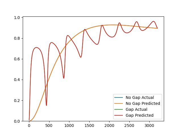
The example below demonstrates another core feature of acoustipy -- optimization routines that are able to identify the JCA model parameters of porous materials from impedance tube measurements. The snippet can also be found under the Inverse Method in the Examples section.
from acoustipy import acousticTMM, AcousticID

# Create an AcousticTMM object to generate toy impedance tube data
structure = acousticTMM(incidence='Normal',air_temperature = 20)

# Define the JCA and air gap material parameters for the toy data
layer1 = structure.Add_JCA_Layer(thickness = 30, flow_resistivity = 46879, porosity = .93, tortuosity = 1.7, viscous_characteristic_length = 80, thermal_characteristic_length = 105)
air = structure.Add_Air_Layer(thickness = 375)

#Generate rigid backed absorption data and save to a csv file
s1 = structure.assemble_structure(layer1)
A1 = structure.absorption(s1)
structure.to_csv('no_gap',A1)

# Generate air backed absorption data and save to a csv file
s2 = structure.assemble_structure(layer1,air)
A2 = structure.absorption(s2)
structure.to_csv('gap',A2)

# Create an AcousticID object, specifying to mount types, data files, and data types
inv = AcousticID(mount_type='Dual',no_gap_file="no_gap.csv", gap_file = 'gap.csv',air_temperature=20,input_type='absorption')

# Call the Inverse method to find the tortuosity, viscous, and thermal characteristic lengths of the material
res = inv.Inverse(30, 47000,.926,air_gap=375,uncertainty=.2,verbose=True)

# Display summary statistics about the optimization
stats = inv.stats(res)
print(stats)

# Plot the results of the found parameters compared to the toy input data
inv.plot_comparison(res)

# Save the optimization results to a csv
inv.to_csv("params.csv",res)

stats = {'slope': 1.000037058594857, 'intercept': 9.276088883464206e-05, 'r_value': 0.9999999674493408, 'p_value': 0.0, 'std_err': 8.732362148426126e-06}